By Ernest Chan and Ray Ng
Optimizing the parameters of a trading strategy via backtesting has one major problem: there are typically not enough historical trades to achieve statistical significance. Whatever optimal parameters one found are likely to suffer from data snooping bias, and there may be nothing optimal about them in the out-of-sample period. That’s why parameter optimization of trading strategies often adds no value. On the other hand, optimizing the parameters of a time series model (such as a maximum likelihood fit to an autoregressive or GARCH model) is more robust, since the input data are prices, not trades, and we have plenty of prices. Fortunately, it turns out that there are clever ways to take advantage of the ease of optimizing time series models in order to optimize parameters of a trading strategy.
One elegant way to optimize a trading strategy is to utilize the methods of stochastic optimal control theory – elegant, that is, if you are mathematically sophisticated and able to analytically solve the Hamilton-Jacobi-Bellman (HJB) equation (see Cartea et al.) Even then, this will only work when the underlying time series is a well-known one, such as the continuous Ornstein-Uhlenbeck (OU) process that underlies all mean reverting price series. This OU process is neatly represented by a stochastic differential equation. Furthermore, the HJB equations can typically be solved exactly only if the objective function is of a simple form, such as a linear function. If your price series happens to be neatly represented by an OU process, and your objective is profit maximization which happens to be a linear function of the price series, then stochastic optimal control theory will give you the analytically optimal trading strategy: with exact entry and exit thresholds given as functions of the parameters of the OU process. There is no more need to find such optimal thresholds by trial and error during a tedious backtest process, a process that invites overfitting to sparse number of trades. As we indicated above, the parameters of the OU process can be fitted quite robustly to prices, and in fact there is an analytical maximum likelihood solution to this fit given in Leung et. al.
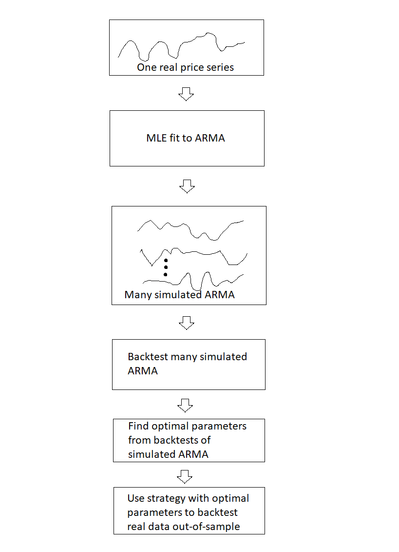
In many optimization problems, when an analytical optimal solution does not exist, one often turns to simulations. Examples of such methods include simulated annealing and Markov Chain Monte Carlo (MCMC). Here we shall do the same: if we couldn’t find an analytical solution to our optimal trading strategy, but could fit our underlying price series quite well to a standard discrete time series model such as ARMA, then we can simply simulate many instances of the underlying price series. We shall backtest our trading strategy on each instance of the simulated price series, and find the best trading parameters that most frequently generate the highest Sharpe ratio. This process is much more robust than applying a backtest to the real time series, because there is only one real price series, but we can we can simulate as many price series (all following the same ARMA process) as we want. That means we can simulate as many trades as we want and obtain optimal trading parameters with as high a precision as we like. This is almost as good as an analytical solution.

Here is a somewhat trivial example of this procedure. We want to find an optimal strategy that trades AUDCAD on an hourly basis. First, we fit a AR(1)+GARCH(1,1) model to the data using log midprices. The maximum likelihood fit is done using a one-year moving window of historical prices, and the model is refitted every month. We use MATLAB’s Econometrics Toolbox for this fit. Once the sequence of monthly models are found, we can use them to predict both the log midprice at the end of the hourly bars, as well as the expected variance of log returns. So a simple trading strategy can be tested: if the expected log return in the next bar is higher than K times the expected volatility (square root of variance) of log returns, buy AUDCAD and hold for one bar, and vice versa for shorts. But what is the optimal K?
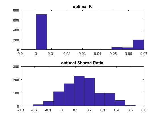
Following the procedure outlined above, each time after we fitted a new AR(1)+GARCH(1, 1) model, we use this to simulate the log prices for the next month’s worth of hourly bars. In fact, we simulate this 1,000 times, generating 1,000 time series, each with the same number of hourly bars in a month. Then we simply iterate through all reasonable value of K and remember which K generates the highest Sharpe ratio for each simulated time series. We pick the K that most often results in the best Sharpe ratio among the 1,000 simulated time series (i.e. we pick the mode of the distribution of optimal K’s across the simulated series). This is the sequence of K’s (one for each month) that we use for our final backtest. Below is a sample distribution of optimal K’s for a particular month, and the corresponding distribution of Sharpe ratios:

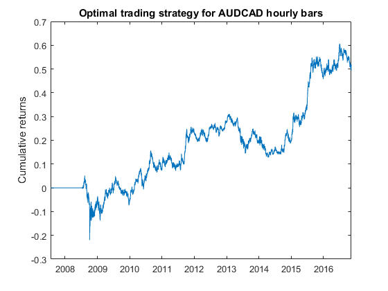
Interestingly, the mode of the optimal K is 0 for any month. That certainly makes for a simple trading strategy: just buy whenever the expected log return is positive, and vice versa for shorts. The CAGR is about 4.5% assuming zero transaction costs and midprice executions. Here is the cumulative returns curve:

You may exclaim: “This can’t be optimal, because I am able to trade AUDCAD hourly bars with much better returns and Sharpe ratio!” Of course, optimal in this case only means optimal within a certain universe of strategies, and assuming an underlying AR(1)+GARCH(1, 1) price series model. Our universe of strategies is a pretty simplistic one: just buy or sell based on whether the expected return exceeds a multiple of the expected volatility. But this procedure can be extended to whatever price series model you assume, and whatever universe of strategies you can come up with. In every case, it greatly reduces the chance of overfitting.
We invented this procedure for our own use a few months ago, borrowing similar ideas from Dr. Ng’s computational research in condensed matter physics systems (see Ng et al here or here). But later on, we found that a similar procedure has already been described in a paper by Carr et al.
About the authors: Ernest Chan is the managing member of QTS Capital Management, LLC. Ray Ng is a quantitative strategist at QTS. He received his Ph.D. in theoretical condensed matter physics from McMaster University.
Upcoming Workshops by Dr. Ernie Chan
November 18 and December 2: Cryptocurrency Trading with Python
I will be moderating this online workshop for Nick Kirk, a noted cryptocurrency trader and fund manager, who taught this widely acclaimed course here and at CQF in London.
February 24 and March 3: Algorithmic Options Strategies
This online course focuses on backtesting intraday and portfolio option strategies. No pesky options pricing theories will be discussed, as the emphasis is on arbitrage trading.

